Feature Importance

Ben Jakubowski
NYU
May 1st, 2018

Learning objectives

Feature Importance

• (Informally) define feature importance, and explain why exploring and presenting feature importance can be both (i) useful, and (ii) potentially misleading.
• Define and describe several feature importance methods that exploit the structure of the learning algorithm or learned prediction function.
• Describe a prediction-function-agnostic method for generating feature importance scores.
• Describe the limitations of these feature importance measures and understand cases where they "fail".

Partial Dependence Plots

• Describe how partial dependence plots are generated.
• Describe the limitations of these plots, and some potential remedies.

Defining feature importance

• Problem setup -- we have some data $(x, y) \in (\mathbb{R}^{d}, \mathcal{Y})$, and a learned prediction function $f$.
• A feature importance method can be loosely understood as a function that maps each feature onto some score.
• These scores rank features by how much they "contribute" to the prediction function $f$.
  • Here "contribute" is defined separately for each method.
  • In general, feature importance is not consistently or rigorously defined.

Why we need to discuss feature importance

• It is easy to compute feature importance from many ML libraries.

Why we need to discuss feature importance

• It is easy to compute feature importance from many ML libraries.
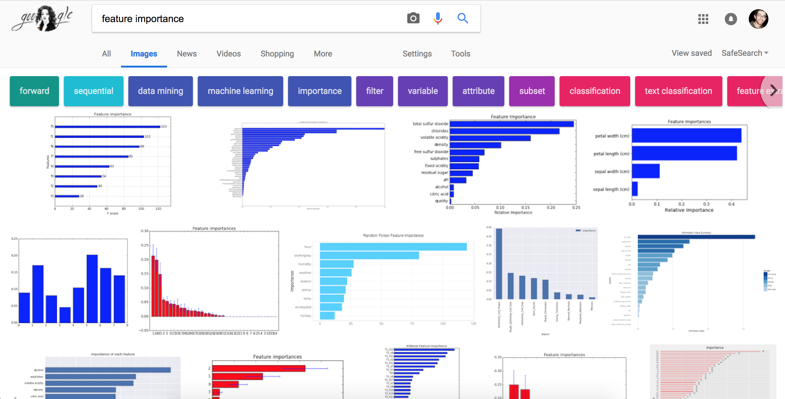
• This means feature importance bar charts show up all over, and it is important to understand:
  • How feature importance can be computed.
  • Potential pitfalls in over interpreting these scores.

Utility of feature importance scores

• Question: Why might feature importance scores be useful?

• Use for sanity checking a model -- do the features that are important seem reasonable, or do they suggest something strange is going on under the hood (i.e. leakage)?

• Share with clients/bosses to build trust and get buy-in on the prediction function.

• Use for feature selection -- can extract the top $K$ features and retrain over this subset (ex: sklearn.feature_selection.SelectFromModel)

Feature selection example

• Breiman's original Random Forests paper showed feature importance for classification of political party based on 16 votes^{[1](https://link.springer.com/content/pdf/10.1023/A:1010933404324.pdf)}:
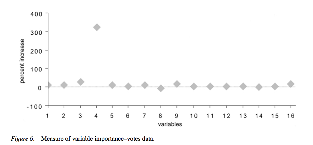
• 'We reran this data set using only variable 4. The test set error is 4.3%, about the same as if all variables were used.'

First example/introducing the issues

• Consider the following feature importance plot for a regression problem with $$\mathcal{Y} = \mathcal{A} = \mathbb{R}, X = \mathbb{R}^{11}$$

hide_code_in_slideshow()
from sklearn.datasets import make_regression
from sklearn.model_selection import train_test_split
from sklearn.linear_model import ElasticNetCV
import pandas as pd
import matplotlib.pyplot as plt
import numpy as np
import seaborn as sns
sns.set_context('notebook', font_scale=1.5)
%matplotlib inline

X,y = make_regression(n_samples=1000, n_features=10,
                      n_informative=3,random_state=1234,
                      shuffle=False, noise=10)
X = np.append(X, X[:,[0]], axis=1)
train_X, test_X, train_y, test_y = train_test_split(X,y,
                                                    test_size=0.2,
                                                    random_state=1235)

enet = ElasticNetCV(l1_ratio=np.array([.1, .5, .7, .9, .95, .99, 1]),
                    n_alphas=500,
                    normalize=True,
                    selection='random',
                    random_state=1351)
enet.fit(train_X, train_y)

coefs = pd.DataFrame({'Feature': np.arange(len(enet.coef_)),
                      'Importance': np.abs(enet.coef_)})
coefs = coefs.set_index('Feature')\
             .sort_values('Importance', ascending=False)
    
fig, ax=plt.subplots(figsize=(12,6))
plot = coefs.plot(kind='bar', title='Example feature importance chart', ax=ax)

• Question: What can we say about this prediction function, it features, and target?

First example/introducing the issues (continued)

• Recall the full feature set includes features $\{0,\cdots,10\}$.
• Let's compare both (a) test set performance ($R^2$), and (b) feature importance plots, for models trained on:
  • All features
  • Features $\{0,\cdots,9\}$
  • Features $\{1,\cdots,9\}$
  • Features $\{1,\cdots,10\}$

First example/introducing the issues (continued)

• Recall the full feature set includes features $\{0,\cdots,10\}$...

from matplotlib import rc
rc('text', usetex=True)

from sklearn.metrics import mean_squared_error
from math import floor

hide_code_in_slideshow()
features_to_test = {
    'All': np.arange(0,11),
    '0-9': np.arange(0,10),
    '1-9': np.arange(1,10),
    '1-10': np.arange(1,11)
}

fig, axarr = plt.subplots(ncols=2, nrows=2, figsize=(12,8))

i = 0
for model_name, features in features_to_test.items():
    col = i % 2
    row = int(floor(i/2))
    
    _train_X = train_X[:, features]
    _test_X = test_X[:, features]
    
    enet = ElasticNetCV(l1_ratio=np.array([.1, .5, .7, .9, .95, .99, 1]),
                        n_alphas=1000,
                        normalize=True,
                        selection='random',
                        random_state=1351)
    enet.fit(_train_X, train_y)

    coefs = pd.DataFrame({'Feature': features,
                          'Importance': np.abs(enet.coef_)})
    coefs = coefs.set_index('Feature')\
                 .sort_values('Importance', ascending=False)

    plot = coefs.plot(kind='bar', title='Typical feature importance chart', ax=axarr[(row,col)])
    
    title = 'Features:' + model_name + r'; $R^2$ =' + \
             str(round(enet.score(_test_X,test_y),3))
    
    axarr[(row,col)].set_title(title)
    
    i += 1
plt.tight_layout()

• What can we learn from this example?

First example/introducing the issues (continued)

• Here was the setup:

  X,y = make_regression(n_samples=1000, n_features=10,
                      n_informative=3, random_state=1234,
                      shuffle=False, noise=10)
  X = np.append(X, X[:,[0]], axis=1)

• Some things to keep in mind:
  • Interactions and correlated/dependent features makes intepretation tricky.
  • Feature importance $\ne$ dependence of target on feature
  • Feature importance $\approx$ contribution of feature to prediction function $f$
  • This doesn't imply there do not exist other functions $f'$ where features that are 'unimportant' in $f$ are 'important'

Where we're headed:

• With this in mind, we're going to look at a number of methods for measuring feature importance.
• We can devide these methods into two basic classes:
  • Algorithmic/prediction-function-specific methods: These exploit the structure of the learning algorithm/prediction function to construct some measure of the relative contribution of each feature.
  • Model agnostic methods: These don't make assumptions on the algorithm or structure of the prediction function; can be applied to any black-box predictor.

Prediction-function-specific: Trees

• Our first algorithm/prediction function specific methods will address decision trees.
• We'll use the Iris Dataset, which is a canonical classification dataset (first used by R.A. Fisher) with:
  • $\mathcal{Y} = $ {Setosa, Versicolour, Virginica} (three varieties of irises).
  • $X = $ [sepal length, sepal width, petal length, petal width] $\in \mathbb{R}^4$

Prediction-function-specific: Trees (Continued)

• Let's consider a shallow tree built on this data.

hide_code_in_slideshow()
from sklearn.datasets import load_iris
from sklearn import tree
import graphviz 

iris = load_iris()
clf = tree.DecisionTreeClassifier(max_depth=3)
clf = clf.fit(iris.data, iris.target)


dot_data = tree.export_graphviz(clf, out_file=None, 
                                feature_names=iris.feature_names,  
                                class_names=iris.target_names,  
                                filled=True, rounded=True,  
                                special_characters=True)  
graph = graphviz.Source(dot_data)  
display.display(graph)

• Question: Which of the feature ([sepal length, sepal width, petal length, petal width]) are most important? Why?

Prediction-function-specific: Trees (Continued)

Tree buiding reminders

• Consider node $t$ in a decision tree built on $N$ training data instances.
• Let node $t$ have $N_t$ node samples.
• We find the split $s_t$ at node $t$ such that $t_L$ and $t_R$ maximizes the decrease $$\Delta i(s, t) = i(t) − p_Li(t_L) − p_Ri(t_R)$$ where $p_L$ and $p_R$ are the probabilities an instance splits left and right, respectively, and $i(t)$ is some some impurity measure.

Prediction-function-specific: Trees (Continued)

Mean decrease impurity

• The mean decrease impurity $imp(X_m)$ for feature $X_m$ is: $$imp(X_m) = \sum_{v(s_t)=X_m}p(t)\Delta i(s_t,t)$$ Note $p(t) = N_t/N$ is the proportion of samples reaching node $t$ and $v(s_t)$ is the variable used in split $s_t$.

Prediction-function-specific: Trees (Continued)

$$imp(X_m) = \sum_{v(s_t)=X_m}p(t)\Delta i(s_t,t)$$

• Question: When will a feature be considered more important under this metric?

• Question: Why is this an algorithm/prediction-function specific method?

Prediction-function-specific: Trees (Continued)

• Implementation:

from collections import defaultdict
import numpy as np

def feature_importance_single_tree(tree, feature_names=iris.feature_names):
    # Returns normed feature importance for a single sklearn.tree
    # Note sklearn trees can handle instance weights, so we need
    # to use weighted_n_node_samples
    
    total_samples = np.sum(tree.weighted_n_node_samples)
    feature_importance = defaultdict(float)
    
    # Identify leaves as described in sklearn's plot_unveil_tree_structure.html
    is_leaf = (tree.children_right == tree.children_left)
    for ix in range(len(is_leaf)):
        if not is_leaf[ix]:
            impurity = tree.impurity[ix]
            split_feature = tree.feature[ix]
            num_at_node = tree.weighted_n_node_samples[ix]

            # Get left child contribution
            left_child = tree.children_left[ix]
            left_decrease = tree.weighted_n_node_samples[left_child]/num_at_node * \
                                tree.impurity[left_child]

            # Get right child contribution
            right_child = tree.children_right[ix]
            right_decrease = tree.weighted_n_node_samples[right_child]/num_at_node * \
                                tree.impurity[right_child]

            delta = impurity - left_decrease - right_decrease
            
            feature_importance[feature_names[split_feature]] \
                += num_at_node / total_samples * delta
    norm = np.sum(feature_importance.values())
    feature_importance = {key: val/norm for key, val in feature_importance.items()}
    return feature_importance

Prediction-function-specific: Trees (Continued)

• Implementation vs. sklearn

imp = feature_importance_single_tree(clf.tree_)
display.display(pd.Series(imp).rename('Importance').to_frame()\
                  .reset_index().rename(columns={'index':'Feature'}))

	Feature	Importance
0	petal length (cm)	0.585616
1	petal width (cm)	0.414384

display.display(pd.DataFrame({'Feature': iris.feature_names,
                              'Importance':clf.feature_importances_})\
                  .sort_values('Importance', ascending=False))

	Feature	Importance
2	petal length (cm)	0.585616
3	petal width (cm)	0.414384
0	sepal length (cm)	0.000000
1	sepal width (cm)	0.000000

Prediction-function-specific: Trees (Continued)

• Question: How do we extend this to ensembles of trees?

• Answer: (Weighted) averages.
  • Ex: Random Forests with $N_T$ trees:

$$Imp(X_m) = \frac{1}{N_T}\sum_T\sum_{t \in T:v(s_t)=X_m}p(t)\Delta i(s_t,t)$$

Prediction-function-specific: Trees (Continued)

• Implementation vs. sklearn

from sklearn.ensemble import RandomForestClassifier
forest = RandomForestClassifier(n_estimators=100) # Not tuned - just example
forest.fit(iris.data, iris.target)
display.display(pd.DataFrame({'Feature': iris.feature_names,
                              'Importance':forest.feature_importances_})\
                  .sort_values('Importance', ascending=False))

	Feature	Importance
2	petal length (cm)	0.449774
3	petal width (cm)	0.433002
0	sepal length (cm)	0.098417
1	sepal width (cm)	0.018807

forest_importance = defaultdict(float)
for tree in forest.estimators_:
    tree_importance = feature_importance_single_tree(tree.tree_)
    
    for key, val in tree_importance.items():
        forest_importance[key] += val
forest_importance = {key:val/len(forest.estimators_)\
                     for key, val in forest_importance.items()}

display.display(pd.Series(forest_importance).rename('Importance').to_frame()\
                  .reset_index().rename(columns={'index':'Feature'})\
                  .sort_values('Importance', ascending=False))

	Feature	Importance
0	petal length (cm)	0.449774
1	petal width (cm)	0.433002
2	sepal length (cm)	0.098417
3	sepal width (cm)	0.018807

Prediction-function-specific: Trees (Continued)

• Let's think about potential variants/extensions to mean decrease impurity.
• How could we handle surrogate splits?

• Commercial implementation of CART adds contributions of surrogate splits:
  • $\Delta i(s_t,t)$ for primary split variable
  • $p^n \Delta i(s_t,t)$ for the $n$'th surrogate split variable (where $p \in [0,1]$ is a user-selected hyperparameter).
• Question: Can we think of any other variants or extensions?

• Consider collapsing the importance of dummy-encoded categoricals.

Prediction-function-specific: Linear models

• Question: How can we measure feature importance in a linear model?

$$imp(X_m) = \big\vert w_m \big\vert$$

• Question: Per usual, how does this notion of importance interact with preprocessing?

Model-agnostic feature importance:

• We've discussed two methods for algorithm or prediction-function specific feature importance measures:
  • Trees (and their ensembles): Mean Decrease Impurity
  • Linear methods: Absolute weights
• Question: How could we determine the importance of input features for an arbitrary black box prediction function?

• Hint 1: Think about defining importance as by measuring how much each feature independently contributes to the performance of the learned model.

• Hint 2: Imagine you were tasked with constructing a synthetic dataset with an unimportant feature -- how could you construct it? Given this insight, what operation could be applied to a feature that would be expected to have (a) no impact on the test set score for unimportant features, and (b) decrease performance for important features?

Model-agnostic feature importance:

Permutation Importance

• Described by Breiman in the original Random Forests paper (using OOB sample).

• We describe it using an arbitrary held-out test set:

  1. Learn prediction function $f$ on training data.
  2. Measure the performance of $f$ on the test set - call this $s_{0}$.
  3. For each feature $i$ in $[1,\cdots,D]$:
     1. Permute just this feature in the test set.
     2. Pass this permuted test set through $f$ to obtain a new score $s_{i}$.
  4. Use either $s_{0} - s_{i}$ (or some appropriate variant on this idea) as feature importance.

Model-agnostic feature importance:

Permutation Importance

• Question: Why bother permuting the feature? Why not just drop it entirely?

• Question: Why bother permuting the feature? Why not replace it with some noise, like $\mathcal{N}(0,1)$?

Model-agnostic feature importance:

Permutation Importance

• Question: Is this any different than the following procedure? If so, how?

  1. Learn prediction function $f$ on training data.
  2. Measure the performance of $f$ on the test set - call this $s_{0}$.
  3. For each feature $i$ in $[1,\cdots,D]$:
     1. Drop this feature from both the training and the test set.
     2. Learn a new prediction function without this feature -- call this function $f_{\setminus i}$
     3. Measure the performance of $f_{\setminus i}$ on the test set to obtain a new score $s_{i}$.
  4. Use either $s_{0} - s_{i}$ as feature importance.

• Key difference: Permutation importance (plus $\big\vert w \big \vert$ and MDI) describe the importance of each feature to a particular prediction function $f$. We don't claim that a feature with low permutation importance in $f$ couldn't have high importance in some other $f'$.

Feature importance pitfalls:

• To conclude our discussion of feature importance, we're going to look at an example to understand potential pitfalls.
• We will compare:
  • Permutation importance
  • MDI for a gradient boosting regressor
  • $\big\vert w \big\vert$ for an elastic net

Feature importance pitfalls: Problem set up

import numpy as np
size = 1000
x1 = np.random.uniform(-10,10,size)
z1 = np.random.uniform(-10,10,size)
x2 = z1 + np.random.normal(0,2,size)
x3 = z1 + np.random.normal(0,2,size)
x4 = z1 + np.random.normal(0,2,size)

def actual_function(x1,z1):
    return -1./2.*x1 + z1 + np.random.normal(0,1,len(x1))

y = actual_function(x1,z1)
X = np.stack([x1,x2,x3,x4]).T

• Question: Which feature is most important (i.e. contributes most to the true conditional mean function)?

• Question: Why might we expect this problem to challenge our feature importance methods?

hide_code_in_slideshow()
corr = pd.DataFrame(X).corr()
corr.index = ['$x_{}$'.format(x) for x in range(4)]
corr.columns = ['$x_{}$'.format(x) for x in range(4)]
display.display(display.Markdown('## Correlation matrix:'))
display.display(corr)

Correlation matrix:

	$x_0$	$x_1$	$x_2$	$x_3$
$x_0$	1.000000	-0.008428	-0.004025	-0.018237
$x_1$	-0.008428	1.000000	0.900929	0.899367
$x_2$	-0.004025	0.900929	1.000000	0.897771
$x_3$	-0.018237	0.899367	0.897771	1.000000

Feature importance pitfalls: Prediction functions

from sklearn.model_selection import train_test_split
from sklearn.ensemble import GradientBoostingRegressor
from sklearn.model_selection import GridSearchCV

train_X, test_X, train_y, test_y = train_test_split(X,y,test_size=0.2,
                                                    random_state=1345134)
reg = GradientBoostingRegressor(n_estimators=200,subsample=0.5,
                                random_state=3141)
grid = GridSearchCV(reg,
                    param_grid={
                        'max_leaf_nodes':[10,25,50],
                        'min_samples_leaf':[10,25,50]
                    }, n_jobs=5, cv=5)
grid = grid.fit(train_X, train_y)

imp = pd.DataFrame({'Feature': ['$x_{}$'.format(i) for i in range(1,5)],
                    'GBM Importance':grid.best_estimator_.feature_importances_})

Feature Importance: Permutation Importance implementation

import eli5
from eli5.sklearn import PermutationImportance

perm = PermutationImportance(grid)
perm.fit(test_X, test_y)

imp['GBM Permutation'] = perm.feature_importances_

Feature Importance: Elastic Net

from sklearn.linear_model import ElasticNetCV

enet = ElasticNetCV(l1_ratio=np.array([.1, .5, .7, .9, .95, .99, 1]),
                    n_alphas=500,
                    normalize=True,
                    selection='random',
                    cv=5,
                    random_state=1351)
enet.fit(train_X, train_y)

imp['Elastic Net $\\vert w \\vert$'] = np.abs(enet.coef_)

perm2 = PermutationImportance(enet)
perm2.fit(test_X, test_y)

imp['Elastic Net Permutation'] = perm2.feature_importances_

Feature Importance: Results

• Recall $E[y~\big\vert~x_1,z] = -\frac{1}{2}x_1+z$. However, we don't observe $z$ -- instead have 3 indepedent noisy observations $x_2,x_3,x_4$. Trying to estimate $E[y~\big\vert~x_1,\cdots,x_4]$

hide_code_in_slideshow()
display.display(imp.set_index('Feature'))

	GBM Importance	GBM Permutation	Elastic Net $\vert w \vert$	Elastic Net Permutation
Feature
$x_1$	0.269611	0.376578	0.493210	0.371113
$x_2$	0.252952	0.163739	0.270237	0.137522
$x_3$	0.240531	0.263513	0.377563	0.257554
$x_4$	0.236906	0.191071	0.307340	0.192642

Feature Importance: Results

• Recall $E[y~\big\vert~x_1,z] = -\frac{1}{2}x_1+z$. However, we don't observe $z$ -- instead have 3 indepedent noisy observations $x_2,x_3,x_4$. Trying to estimate $E[y~\big\vert~x_1,\cdots,x_4]$

hide_code_in_slideshow()
sns.set_context('notebook',font_scale=2)
fig, ax = plt.subplots(figsize=(12,8))
plot = imp.set_index('Feature').plot(kind='bar', ax=ax)

• What are the implications, and what can we learn from this experiment?

Partial Dependence Plots

• Imagine we have a subset of features we think are important.
  • This could be based on "feature importance" scores or coefficients, or other reasons (i.e. prior knowledge/research questions/etc.).
  • We may want to dig deeper to explain the relationship between our predictions and these features.
  • Question: Why? If we have MDI feature importance scores in hand, what do we not know?

• Directionality:
  • Note in reality we probably have complex, non-monotonic relationships
  • However even if we have a monotonic relationship, or even linear, our MDI wouldn't give any indication on the direction -- obviously weights in a linear model would.
• Partial dependence plots let us dig deeper and visualize the dependence of our prediction function (i.e. predict/predict_proba) on one or two of these features.

Partial Dependence Plots: Setup

• Consider an arbitrary prediction function $f$ learned over a training set $\mathcal{D}$.

• This dataset includes $N$ observations $y_i$ of a target $y$ for $i = 1,2,\cdots,N$, along with $p$ features denoted $x_{i,j}$ for $j=1,2,\cdots,p$ and $i=1,2,\cdots,N$. This model generates predictions of the form: $$\hat{y}_i = f(x_{i,1},x_{i,2},\cdots,x_{i,p})$$

• In the case of a single feature $x_j$, Friedman's partial dependence plots are obtained by computing the following average and plotting it over a useful range of $x$ values: $$\phi_j(x) = \frac{1}{N}\sum_{i=1}^N f(x_{i,1},\cdots,x_{i,j-1},x,x_{i,j+1},\cdots,x_{i,p})$$

• PDPs for more than one variable are computed (and plotted) similarly.
• Question: What would $\phi_j(x)$ be for a linear prediction function?

Partial Dependence Plots: Setup

$$\phi_j(x) = \frac{1}{N}\sum_{i=1}^N f(x_{i,1},\cdots,x_{i,j-1},x,x_{i,j+1},\cdots,x_{i,p})$$

• Question: Think about $\phi_j(x)$ -- what issues can we already anticipate?

• Imagine $P(x_j = x_{j+1}) = 1$. Then even though there is zero density where $x_j \ne x_{j+1}$, we still can evaluate $\phi_j(x)$ at $x \ne x_{i, j+1}$ for all $i \in {1,\cdots,n}$.
• Previewing what's next: Think about the potential impact of taking the average $\frac{1}{N}\sum_{i=1}^N (\cdot) $

PDP Example: California Housing

• Example derived from sklearn PDP example, using sklearn utilities.
• While not shown, we first train a GBM on the California Housing dataset:

hide_code_in_slideshow()
print(cal_housing.DESCR)

California housing dataset.

The original database is available from StatLib

    http://lib.stat.cmu.edu/datasets/

The data contains 20,640 observations on 9 variables.

This dataset contains the average house value as target variable
and the following input variables (features): average income,
housing average age, average rooms, average bedrooms, population,
average occupation, latitude, and longitude in that order.

References
----------

Pace, R. Kelley and Ronald Barry, Sparse Spatial Autoregressions,
Statistics and Probability Letters, 33 (1997) 291-297.

PDP Example: California Housing

• Example derived from sklearn PDP example, using sklearn utilities.
• While not shown, we first train a GBM on the California Housing dataset:

hide_code_in_slideshow()
fig, ax = plt.subplots(figsize=(12,6))
plot = pd.Series(reg.feature_importances_,
                          index=names).rename('MDI').to_frame()\
                  .sort_values('MDI', ascending=False).plot(kind='bar',ax=ax,
                                                            title='Importance: Mean Decrease Impurity')

PDP Example: California Housing

• Next, we present the PDPs for several single features, and one pair of features.

hide_code_in_slideshow()
features = [0, 5, 1, 2, (5, 1)]
fig, ax = plt.subplots(figsize=(12,10))
fig, ax = plot_partial_dependence(reg, X_train, features,
                                  feature_names=names,
                                  n_jobs=3, grid_resolution=50,
                                  ax=ax)
fig.suptitle('Partial dependence of house value on nonlocation features')
plt.subplots_adjust(top=0.9)  # tight_layout causes overlap with suptitle
plt.show()

PDP Example: California Housing

• Note we don't plot the spatial features -- in fact, what would perhaps be most interesting (and a potential optional extension for indidivual exploration) would be to plot the long/lat PDP over a base map.
  • An easy python first pass might simply use geopandas.

PDP Pitfalls:

• Consider the following PDP for a regression problem with $\mathcal{Y} = \mathbb{R}$ and $X = \mathbb{R}^3$.

hide_code_in_slideshow()
fig, ax = plt.subplots(figsize=(12,8))
plot_partial_dependence(grid.best_estimator_, Xs, [1],
                        n_jobs=1, grid_resolution=25, ax=ax)
plt.xlim(-1,1)
plt.ylim(-6,6)
plt.xlabel('$X_1$')

pass

• Question: What can we learn about the relationship between feature $X_2$ and our target $Y$?

PDP Pitfalls:

• Here was the data generating process:

size = 10000
X1 = np.random.uniform(-1,1,size)
X2 = np.random.uniform(-1,1,size)
X3 = np.random.uniform(-1,1,size)
eps = np.random.normal(0,0.5,size)
Y = 0.2*X1 - 5*X2 + 10*X2*np.where(X3>=0,1,0) + eps

Xs = np.stack([X1,X2,X3]).T

hide_code_in_slideshow()
fig, ax = plt.subplots(figsize=(12,8))
plt.scatter(X2[X3>=0], Y[X3>=0], color='blue', label='$X_3>=0$')
plt.scatter(X2[X3<0], Y[X3<0], color='green', label='$X_3<0$')
plt.ylabel('$Y$')
plt.xlabel('$X_2$')
plt.legend()
plt.show()

PDP Pitfalls:

• Recall $$y = 0.2 x_1 - 5 x_2 + 10 x_2 \mathbb{1}(x_3 >= 0) + \varepsilon$$
• Question: Why does the PDP fail to reveal the dependence of $y$ on $x_2$?

In his gradient boosting paper, Friedman identified this issue (here presented in our notation):

• In general, the functional form of $\phi_j(x)$ will depend on the particular values chosen for $\setminus j$. If, however, this dependence is not to strong than the average function can represent a useful summary of the partial dependence of $f$ on the chosen variable subset $j$.

PDP Pitfalls: Another option

• One response to this shortcoming has been development of "Individual Conditional Expectation" plots -- see Goldstein et al, 2014.
• Their insight was that taking an average is a post-processing step that can mask structure.
• We'll use the SauceCat/PDPbox implementation.

hide_code_in_slideshow()
from pdpbox import pdp

train = pd.DataFrame(Xs)
train.columns = [str(x) for x in train.columns]

pdp_one = pdp.pdp_isolate(grid, train, '1')
pdp.pdp_plot(pdp_one, '$x_1$',
             plot_org_pts=True, plot_lines=True,
             center=False, frac_to_plot=1000)

• Question: Note the average (i.e. classic PDP plot) is shown in yellow. How do the additional traces aide clarify the dependence of $y$ on $x_1$?

Next steps

• We started by talking about feature importance.
  • This gave a set of methods for trying to build insight into how much each feature contributed to the prediction function -- though we saw this is somewhat ill-defined. It didn't give insight into even the directionality of simple linear relationships -- let alone more complex stucture.

• Next we looked at PDPs
  • PDPs give some insight into average relationship between one or two predictors and the target. However, this was shown to be potentially misleading, if the average relationship masks interactions.

• This led us to ICEplots, which plot a trace for each data instance separately.

• Note this trajectory (moving from global to data-instance-specific measures of importance) could be extended -- next steps might look at additive feature attribution methods such as SHAP values.

Bibliography

Papers

• Brieman, L (2001). Random Forests.
• Friedman, J (2001). Greedy Function Approximation: A Gradient Boosting Machine.
• Goldstein et al (2014). Peeking Inside the Black Box: Visualizing Statistical Learning with Plots of Individual Conditional Expectation

Packages

• scikit-learn/scikit-learn
• TeamHG-Memex/eli5
• SauceCat/PDPbox